Model formulation and parameter estimation

Model-based Geostatistics for Global Public Health

Emanuele Giorgi

Lancaster University

Overview of topics

How to assess residual spatial correlation
How to formulate and fit a geostatistical model
How to interpret the results from a model fit

Which residuals should we use to assess spatial correlation?

Pearson Residuals: \[\frac{y_i - \hat{y}_i}{\sqrt{\text{Var}(\hat{y}_i)}}\]
Deviance Residuals: \[\text{sign}(y_i - \hat{y}_i) \times \sqrt{d_i}\] where \(d_i\) is the deviance contribution of observation \(i\).
Random Effects Residuals: \(\hat{Z}_i\), i.e. the estimated random effect for each location/household/cluster/village.

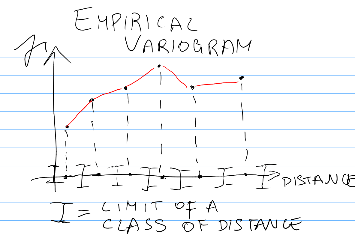
The Empirical Variogram using Random Effects Residuals

The empirical variogram is defined as: \[ \gamma(D_{[a,b]}) = \frac{1}{2|D_{[a,b]}|} \sum_{(i,j) \in D_{[a,b]}} (\hat{Z}_i - \hat{Z}_j)^2 \] where:
- \(D_{[a,b]}\) is a class of distance with lower limit \(a\) and upper limit \(b\);
- \(|D_{[a,b]}|\) is the number of pairs of observations whose locations ar at a distance between \(a\) and \(b\).

liberia_variog.R

Stationary and Isotropic Gaussian Processes

A Gaussian Process (GP) is a collection of random variables, any finite subset of which follows a multivariate normal distribution.
A GP is stationary if its statistical properties do not change with location shifts.
It is isotropic if its properties do not change with locations rotations.
We denote a GP as \(S(x)\), where \(x\) represents location.
For a stationary and isotropic GP, the correlation function is purely a function of the distance between locations.

The Matérn Process

The Matérn covariance function is the most widely used in geostatistics.
It is controlled by three parameters:
- Variance (\(\sigma^2\)) – controls process magnitude
- Smoothness (\(\kappa\)) – determines differentiability
- Scale parameter (\(\phi\)) – governs spatial correlation decay
The covariance function is given by: \[ C(h) = \sigma^2 \frac{2^{1-\kappa}}{\Gamma(\kappa)} \left( h/\phi \right)^\kappa K_\kappa \left(h/\phi \right), h = ||x-x'|| \] where \(K_\kappa\) is the modified Bessel function of the second kind.

matern_simulator.R

Special Cases of the Matérn Covariance

The Matérn family includes two important special cases:

Exponential Covariance (\(\kappa = 1/2\))
\[ C(h) = \sigma^2 \exp\left(-\frac{h}{\phi}\right) \]
Properties:
- Relatively rough process, non-differentiable
- Continuous but not differentiable
- Markovian (memoryless) property

Gaussian (Squared Exponential) Covariance (\(\kappa \to \infty\))
\[ C(h) = \sigma^2 \exp\left(-\frac{h^2}{2\phi^2}\right) \]
Properties:
- Infinitely differentiable
- Produces very smooth realizations
- Sometimes too smooth for physical processes

Practical Range of Spatial Correlation

Definition: Distance (\(h^*\)) where correlation drops to 0.05 (5%)
- Represents the effective spatial dependence range
- Commonly used cutoff in geostatistics
General Solution: \[ \rho(h^*) = 0.05 \] Solve for \(h^*\) to find practical range
Exponential Covariance Example: \[ \rho(h^*) = \exp\left(-\frac{h^*}{\phi}\right) = 0.05 \] \[ \Rightarrow -\frac{h^*}{\phi} = \log(0.05) \approx -3 \] \[ \Rightarrow h^* \approx 3\phi \]
- Practical range: \(3\phi\)
- At \(h^* = 3\phi\), correlation drops to ~5%

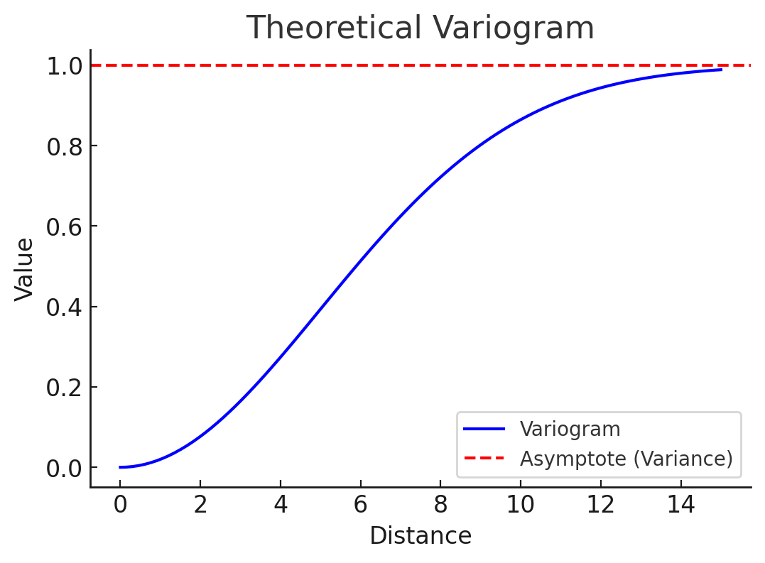
Theoretical Variogram

The variogram measures spatial dependence: \[ \gamma(h) = \frac{1}{2} \mathbb{E} \left[\left\{S(x) - S(x')\right\}^2\right] \]
For the Matérn process, it is derived from its covariance function \[ \gamma(h) = \sigma^2 \left( 1 - \rho(h) \right), h = ||x-x'|| \] where \(\rho(h)\) is the correlation function of \(S(x)\).

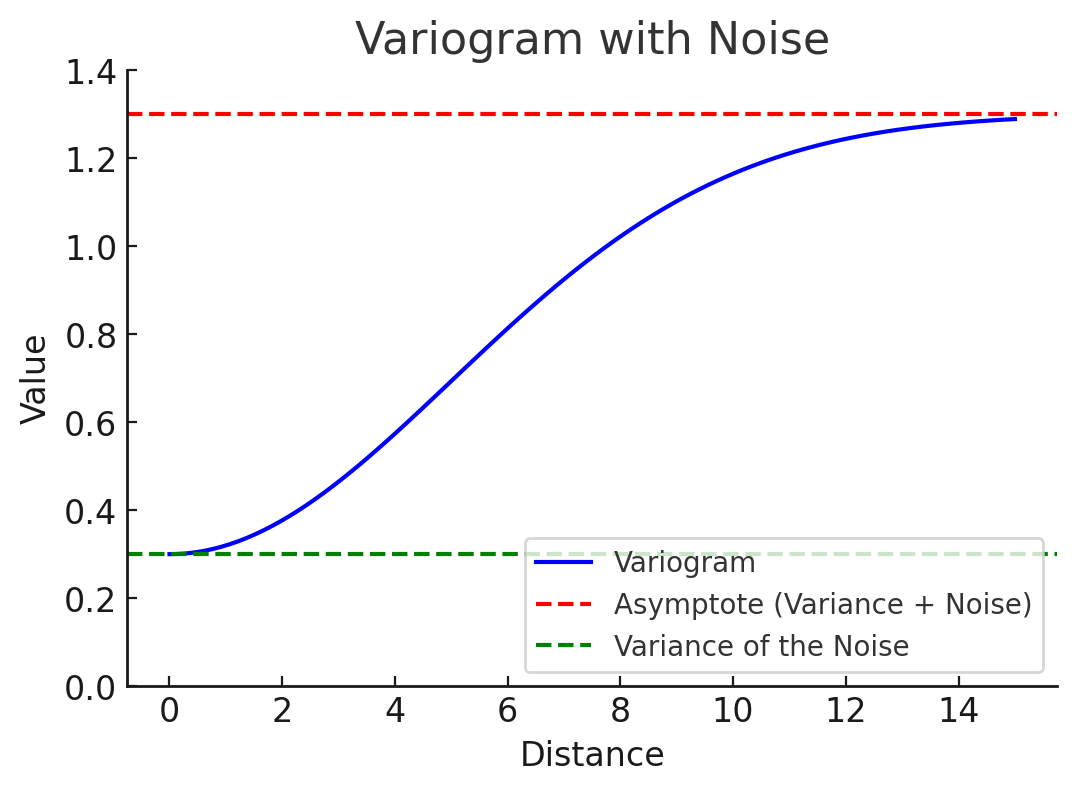
Theoretical Variogram with Noise

The variogram measures spatial dependence: \[ \gamma(h) = \frac{1}{2} \mathbb{E} \left[\left\{S(x) + Z(x) - S(x') - Z(x')\right\}^2\right] \]
Where \(Z(x)\) is Gaussian noise with mean 0 and variance \(\tau^2\)
The expression of the variogram changes to \[ \gamma(h) = \tau^2 + \sigma^2 \left( 1 - C(h) \right), h = ||x-x'|| \] . . .

The linear geostatistical model

The general expression is

\[ Y_i = d(x_i)\top \beta + S(x_i) + U_i \]

where: \(d(x_i)\) are covariates, \(S(x_i)\) is a stationary and isotropic spatial Gaussian process and \(U_i\) is Gaussian noise.

Denote \(S = (S(x_1), \ldots, S(x_n))\).

Assuming \(R(\phi)\) to be the correlation matrix of \(S\), and \(U_i \sim \text{N}(0, \tau^2)\), the vector of observations \(\mathbf{Y} = (Y_1, \dots, Y_n)^T\) follows a multivariate normal distribution:

\[ \mathbf{Y} \sim \text{MVN}\left(D\beta, \Sigma\right) \]

where the covariance matrix is given by

\[ \Sigma = \sigma^2 R(\phi) + \tau^2 I_n. \]

Parameter Estimation via Likelihood

The parameters \(\theta = (\mu, \sigma^2, \tau^2, \phi)\) are estimated by maximizing the log-likelihood function:

\[ \ell(\theta) = -\frac{1}{2} \left[ n \log(2\pi) + \log |\Sigma| + (\mathbf{Y} - D\beta)^T \Sigma^{-1} (\mathbf{Y} - D\beta) \right]. \]

Optimization is typically performed using numerical methods such as gradient-based algorithms or derivative-free approaches like the Nelder-Mead method.

Using moss to monitor air pollution

galicia_fit.R

Generalized linear geostatistical models

Let \(S(x)\) be a stationary and isotropic Gaussian process, with Matérn correlation function.

Let \(Z_i\) be independent identically distributed random variables.

Let \(d(x_i)\) be a vector of covariates with associated regression coefficients \(\beta\).

Let \(Y_i\) be a random variable that, conditionally on \(S(x_i)\) and \(Z_i\), follows an exponential family distribution (e.g. Gaussian, Binomial, Poisson).

Let \(g(\cdot)\) be a link function.
- \(\mathbb{E} \left[ Y_i \: | \: S(x_i), Z_i \right] = m_i \mu_i\)
- \({\rm Var}\left[Y_i \: | \: S(x_i), Z_i\right] = m_i V(\mu_i)\)
- \(g(\mu_i) = d(x_i)^\top \beta + S(x_i) + Z_i\)

Binomial and Poisson Geostatistical Models

Binomial Geostatistical Model
- \(Y_i \: | \: S(x_i), Z_i \sim \text{Binomial}(m_i, \mu_i)\)
- Link function: Logit link \(g(\mu_i) = \log \left( \frac{\mu_i}{1 - \mu_i} \right) = d(x_i)^\top \beta + S(x_i) + Z_i\)
- Variance function: \(V(\mu_i) = m_i \mu_i (1 - \mu_i)\)

Poisson Geostatistical Model
- \(Y_i \: | \: S(x_i), Z_i \sim \text{Poisson}(m_i \mu_i)\)
- Link function: Log link \(g(\mu_i) = \log (\mu_i) = d(x_i)^\top \beta + S(x_i) + Z_i\)
- Variance function: \(V(\mu_i) = m_i \mu_i\)

Monte Carlo Maximum Likelihood (MCML)

Let \(W_i = S(x_i) + Z_i\) and \(W = (W_1, \ldots, W_n)\)

The likelihood function for parameters \(\theta = (\beta, \sigma^2, \phi, \tau^2)\) is given by:

\[ L(\theta) = \int N(W; D\beta, \Omega) f(y| W) dW \]

where \(\Omega = \sigma^2 R(\phi) + \tau^2I_n\).

We approximate this using Monte Carlo integration:

\[ L_m(\theta) = \frac{1}{B} \sum_{j=1}^{B} \frac{N\left(W^{(j)}; D\beta, \Omega \right)}{N\left(W^{(j)}; D\beta_0, \Omega_0\right)} \] where \(W^{(i)}\) are sampled from the distribution of \(W\) given \(y\) using an MCMC algorithm.

MCML: Iterative Estimation

Choose initial values \(\theta_0\) and generate samples \(W^{(j)}\), for \(j = 1,\ldots, B\).

Estimate \(\theta\) by maximizing the Monte Carlo approximation, denoted by \(L_m(\theta)\), to the likelihood. Denote with \(\hat{\theta}_m\) this estimate.

Update \(\theta_0 = \hat{\theta}_m\) and iterate until convergence.

Standard errors are computed using the inverse Hessian of \(L_m(\theta)\) at \(\hat{\theta}_m\).

glgm_fit.R

The Nugget Effect as Small-Scale Spatial Correlation

Interpretation of \(Z_i\):
- Represents microscale variation (below measurement distance)
- Captures measurement error or sub-resolution variability
Example Process with Threshold Correlation: \[ \rho(h) = \begin{cases} \delta & \text{if } h \leq h_0 \\ 0 & \text{if } h > h_0 \end{cases} \]
- Where \(\delta\) is small-scale correlation
- \(h_0\) is resolution threshold
Practical Implications:
- If minimum distance between samples \(> h_0\):
  - Process appears as \(Z_i \sim N(0, \tau^2)\) (pure noise)
  - Spatial structure in \(Z_i\) becomes undetectable
- Cannot disentangle \(Z_i\) from measurement error in the lineara geostatistical model