Exploratory analysis

Model-based Geostatistics for Global Public Health

Emanuele Giorgi

Lancaster University

Overview of topics

• How to explore relationships with count data
• How to use a non-spatial model for mapping
• How to handle spatial data in R

Exploring relationships

• How to explore relationships with count data (binary and aggregated counts)?
• How to model non-linear relationships?
• How to use a non-spatial model for mapping?

explore_associations.R

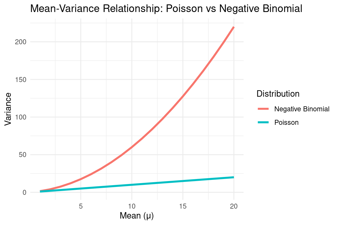
Overdispersion in Count Data

• What is overdispersion?
  • Occurs when the variance of count data exceeds the mean.
  • Violates the Poisson assumption:
    \[ \text{Var}(Y) = \mathbb{E}(Y). \]
• Why does it matter?
  • Standard models (e.g., Poisson regression) underestimate uncertainty.
  • Leads to overly optimistic confidence intervals and p-values.

Example: Overdispersion in Correlated Binary Data

• Consider \(Y = \sum_{i=1}^n X_i\), where \(X_i\) are correlated binary variables.

• If \(X_i\) are independent, \(Y\) follows a Binomial distribution: \[ \mathbb{E}(Y) = np, \quad \text{Var}(Y) = np(1-p). \]

• If \(X_i\) are correlated, the variance increases:
  \[ \text{Var}(Y) = np(1-p) + \sum_{i \neq j} \text{Cov}(X_i, X_j). \]

• This leads to overdispersion.

Example: Negative Binomial Distribution

• A common solution for overdispersed count data.

• Extends the Poisson distribution by introducing a dispersion parameter \(\alpha\):
  \[ \mathbb{E}(Y) = \mu, \quad \text{Var}(Y) = \mu + \alpha \mu^2. \]

• When \(\alpha = 0\), it reduces to Poisson.

• Random Effects Interpretation:

  • The Negative Binomial can be interpreted as a Gamma-Poisson mixture.
  • The Poisson mean \(\mu\) is drawn from a Gamma distribution, introducing extra variability.

Random Effects Models for Overdispersion

• Overdispersion often arises due to unobserved heterogeneity.
• A solution is to introduce random effects that account for latent variability.

• Random Intercept Model:
  \[ Y_{ij} \mid b_j \sim \text{Poisson}(\mu_{ij}), \quad \log(\mu_{ij}) = X_{ij} \beta + b_j. \]

• \(b_j \sim \mathcal{N}(0, \sigma^2)\) captures between-group variability.

• Leads to extra variability in counts, addressing overdispersion.

• Connection to Negative Binomial:
  • If \(b_j\) follows a Gamma distribution instead of Normal, the model is equivalent to a Negative Binomial.

Marginal Models for Overdispersion

• An alternative to random effects models is using marginal models.

• Instead of modeling subject-level variation, these models estimate population-averaged effects.

• Generalized Estimating Equations (GEE):

  • Does not assume a specific distribution for random effects.
  • Uses a working correlation matrix to account for within-group dependence.
  • Robust standard errors help correct for overdispersion.

See Diggle, Heagerty, Liang, Zeger

Choosing Between Models

Comparison of Random Effects vs. Marginal Models
Feature	Random Effects Model	Marginal Model (GEE)
Interpretation	Subject-specific	Population-averaged
Handles Overdispersion	Yes (via latent effects)	Yes (via robust SE)
Computational Complexity	Higher	Lower

Example 1

• A clinical trial measuring blood pressure at multiple time points for patients in different hospitals.
  
• Why Use Random Effects?
  • Each patient has their own baseline blood pressure that varies.
    
  • A random intercept accounts for individual differences.
    
  • If hospitals have different treatment protocols, a random hospital effect can be included.

Example 2

• Study Design: A population-wide study on whether a new influenza vaccine reduces hospitalization rates.
  
• Why Use Marginal Models?
  • Interest is in the population-averaged effect of the vaccine, not individual variation.
    
  • Generalized Estimating Equations (GEE) account for correlation in repeated measures without assuming a specific random effect structure.

A class of generalized linear models

Assumptions:

1. \(Z_{i}\) are i.i.d. random variables;

2. \(Y_{i} \mid Z_i \sim f(\cdot)\) belongs to the exponential family;

3. \(E[Y_{i}\mid Z_i] = m_i \mu_{i}\) and \(\text{Var}[Y_{i} \mid Z_i] = m_i V(\mu_{i})\);

4. \(g(\mu_{i}) = \eta_i = d_i^\top \beta + Z_i\);

5. \(Y_i \mid Z_i\) are mutually independent for \(i=1,\dots,n\).

Parameter Estimation

• Likelihood function

The vector of unkown parameters is \(\theta=(\beta, \sigma^2)\) \[ L(\theta) = \prod_{i=1}^n \int_{-\infty}^{+\infty} [Z_i] [Y_i \mid Z_i] \: dY_i \]

• Estimation Method

Maximize the likelihood using the Laplace approximation (glmer in the lme4 package).

• Hypothesis Testing

  1. Obtain \(\hat{\theta}\) (MLE).
  2. Obtain \(\hat{\theta}_{0}\), the MLE constrained by fixing \(p\) values of \(\beta\) to 0.
  3. Compute the log-likelihood ratio:

  \[ D = 2(\log L(\hat{\theta}) - \log L(\hat{\theta}_0)) \sim \chi^2_{p} \]

  4. P-value: \(P(D > D_{obs} \mid H_0)\)

Example: Riverblindness in Liberia

glmer_fit.R

Coordinate Reference Systems (CRS)

Geographic vs. Projected CRS

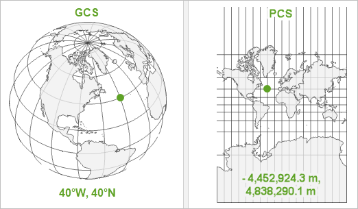
• A CRS defines how spatial data is projected onto the Earth’s surface.
• Two main types:
  • Geographic CRS (Latitude/Longitude, e.g., WGS84)
  • Projected CRS (e.g., UTM, which uses meters for measurements)

Computing Distance

• Distances in Geographic CRS (Lat/Lon) require geodesic calculations (e.g., Haversine formula).

• Projecting to UTM allows for Euclidean distance calculations in meters.

• Conversion to UTM in R:

  library(sf)
  points <- st_as_sf(data.frame(lon = c(-0.1, -0.2), lat = c(51.5, 51.6)), 
                     coords = c("lon", "lat"), crs = 4326)
  points_utm <- st_transform(points, crs = 32630)

Spatial Data Formats

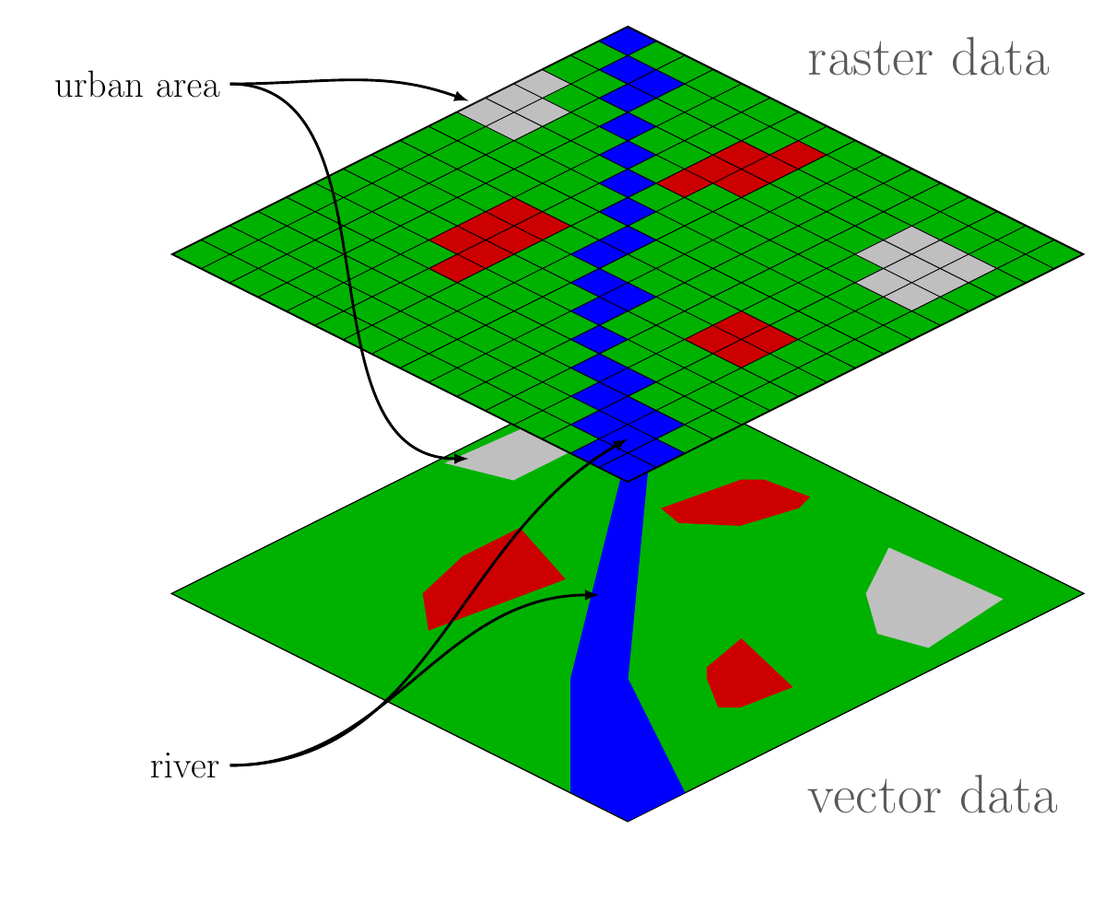
• Shapefiles:
  • Vector data format for storing geometries (points, lines, polygons).
  • Commonly used in GIS applications.
• Raster Files:

  • Grid-based data (e.g., satellite images, elevation models).

  • Each cell has a value representing an attribute (e.g., temperature, elevation).

Mapping with covariates only {.smaller]}

Consider the following GLMM for the Liberia data on riverblindness. \[ \log\left\{\frac{p(x_i)}{1-p(x_i)}\right\} = \beta_0 + \beta_1 \log\{e(x_i)\} + Z_i \] where \(e(x)\) is the elevation in meters at location \(x\) and \(Z_i \sim N(0,\tau^2)\) i.d.d.

Question: How can we use this model for mapping?

glmm_mapping.R