Geostatistical prediction
Model-based Geostatistics for Global Public Health
Geostatistical problems
“Conventional geostatistical methodology solves the problem of predicting the realized value of a linear functional of a Gaussian spatial stochastic process \(S(x)\) based on observations \(Y_i= S(x_i) + Z_i\) at sampling locations \(x_i\), where the \(Z_i\) are mutually independent, zero-mean Gaussian random variables.”
Defining the predictive target
. . .
- Spatially continuous targets correspond to an unobserved spatially continuous surface (e.g. disease prevalence), formally denoted by \(\mathcal{T} = \{T(x), x \in A\}\), where \(A\) is our region of interest.
. . .
- Areal-level targets, usually defined as transformation of the spatially continuous surface \(\mathcal{T}\), defined previously, and which we denote as \(\mathcal{T}_{A} = F(\mathcal{T}, A)\).
Examples of predictive target
| Predictive target \(T(x)\) | Name | GLM family |
|---|---|---|
| \(d(x)^\top \beta + S(x)\) | Linear predictor | Any GLM |
| \(\frac{\exp\{d(x)^\top \beta + S(x)\}}{1+\exp\{d(x)^\top \beta + S(x)\}}\) | Prevalence | Binomial |
| \(\exp\{d(x)^\top \beta + S(x)\}\) | Mean number of cases | Poisson |
| \(S(x)\) | Spatial random effects | Any GLM |
| \(d(x)^\top \beta\) | Covariates effects | Any GLM |
The predictive distribution of the target
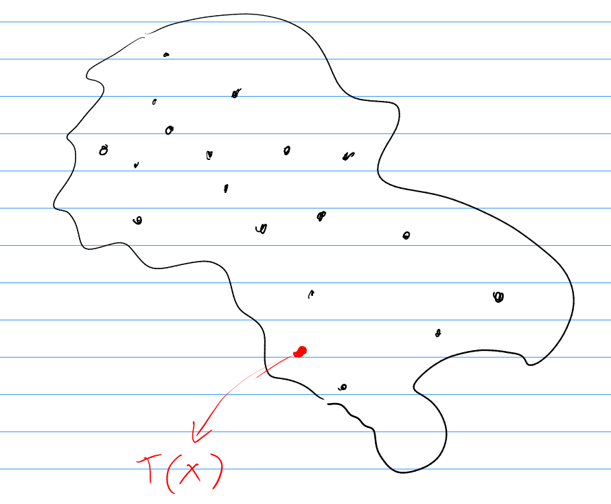
The predictive distribution of the target
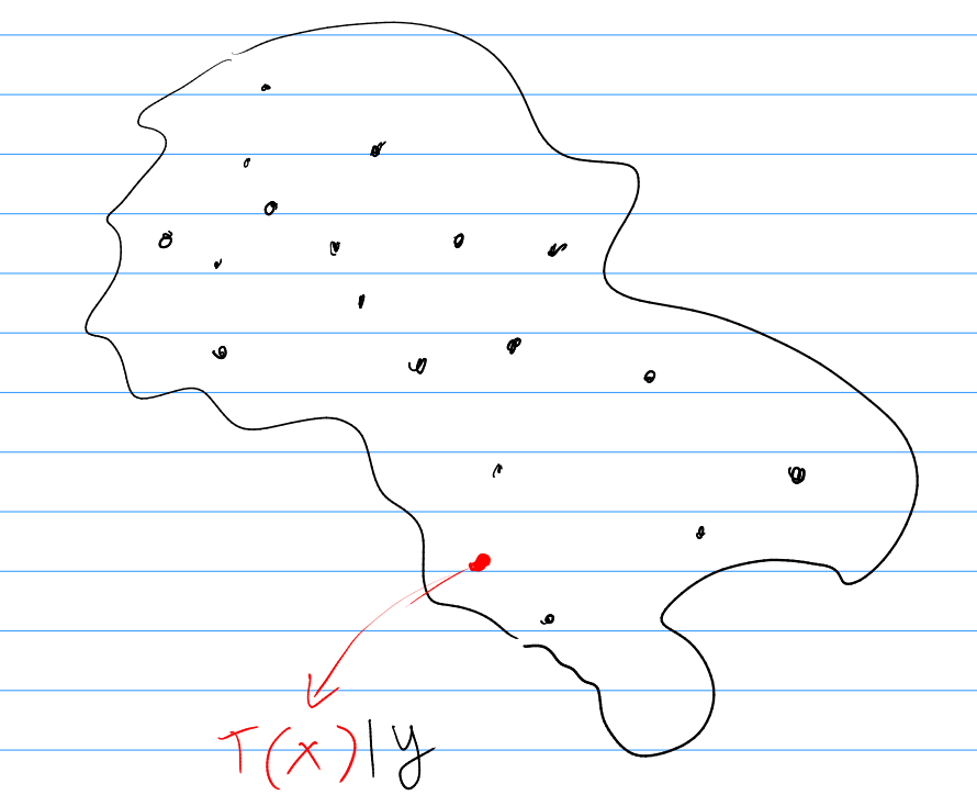
The predictive distribution of the target
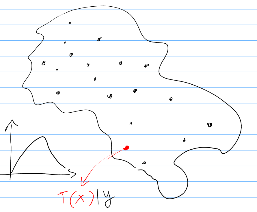
The predictive distribution of the target
The predictive distribution of the target
Steps for the geostistical prediction of \(T(x)\)
Preliminary steps:
- Obtain the shapefile of the boundaries of the study area.
- Generate a regular grid that covers the study for the desired spatial resolution, using the shapefile.
- Extract all the covariates used in the model on the grid and ensure that there are no missing values.
. . .
Prediction steps (for a given location \(x\) on the grid):
- Generate samples from the predictive distribution of \(S(x) \: | \: y\), say \(S_{(j)}(x)\), for \(j = 1, \ldots, B\).
. . .
- Apply the transformation defined by \(T(x)\) to each of the samples \(S_{(j)}(x)\), to obtain \(T_{(j)}(x)\), for \(j = 1, \ldots, B\).
. . .
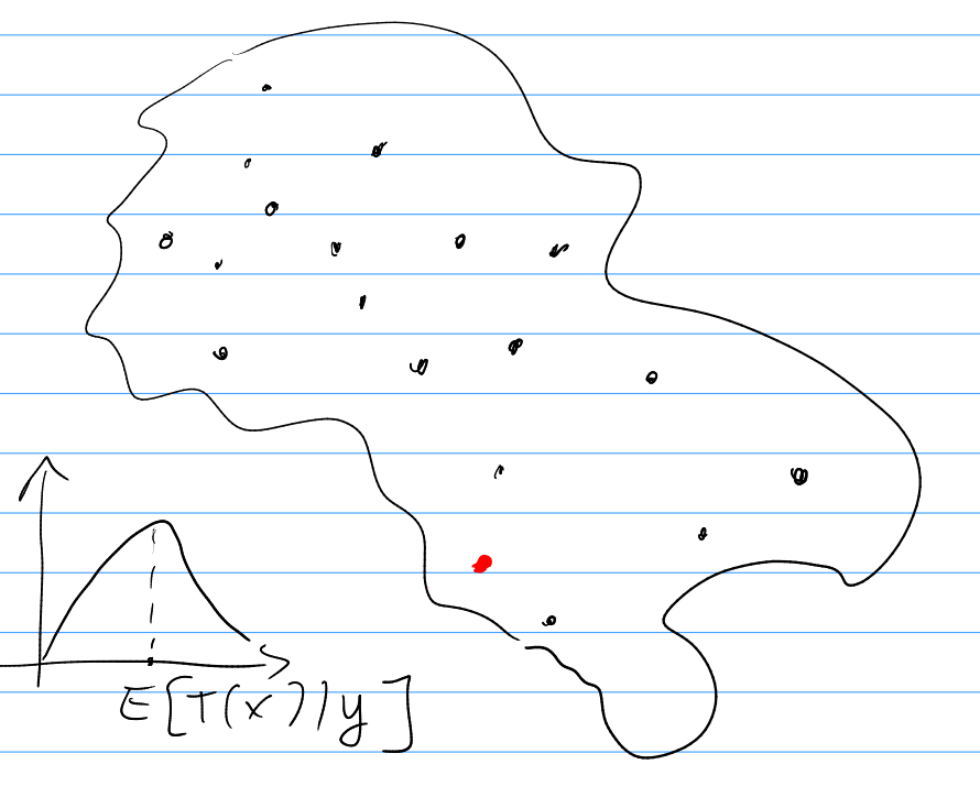
Using the Monte Carlo samples \(T_{(j)}(x)\), obtain the desired summaries of the predictive distribution:
Mean: \(\overline{T}_B = B^{-1} \sum_{j=1}^B T_{(j)}(x)\)
Standard deviation: \(\left[B^{-1} \sum_{j=1}^B (T_{(j)}(x) - \overline{T}_B)^2\right]^{1/2}\)
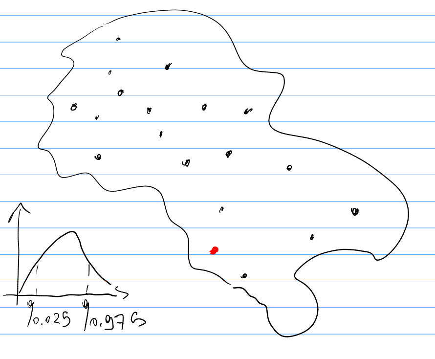
Prediction intervals at 95\(\%\) coverage level
Exceedance probabilities: \(B^{-1} \sum_{j=1}^B I(T_{(j)}(x) > L)\), for a given threshold \(L\).
. . .

Marginal vs joint predictions
- Let \(\tilde{X} = (\tilde{x}_1, \ldots, \tilde{x}_q)\) be the set of prediciton locations that are make up the regular grid.
. . .
- Marginal predictions are obtained by simulating independently from the \(q\) marginal predictive distributions of \([S(\tilde{X}) | y]\). In other words, we consider a prediction location \(\tilde{x}_j\), simulate from \([S(\tilde{x}_j) \: |\: y]\) say \(B\) samples, and repeat this for \(j=1,\ldots,q\)
. . .
- Joint predictions are obtained by simulating from the joint distribution of \([S(\tilde{X}) \: |\: y]\). Unlike marginal predictions, joint predictions take into account the correlation between the different components of \([S(\tilde{X}) \: |\: y]\).
. . .
- When the target is \(T(x)\), i.e. at pixel-level, we can use either marginal or joint predictions.
. . .
- When the target is areal level (see next slides), we can ONLY use joint predictions.
Areal-level targets: questions to consider
- What spatially continuous target, \(T(x)\), are we seeking to aggregate?
- What are the spatial units, denoted as \(A_i\) for \(i = 1, \dots, N\), over which the aggregation is required?
- What aggregating function should be applied?
- Should spatial weights be incorporated in the aggregation, and if so, what weights are appropriate?
Example: regional average prevalence
- Let \(T(x) = \exp\{d(x)^\top \beta + S(x) \}/(1+\exp\{d(x)^\top \beta + S(x)\})\)
. . .
- Average (unweighted) prevalence \[ \mathcal{M}_i = \frac{1}{|A_i|}\int_{A_i} T(x) \: dx. \]
. . .
- Average weighted prevalence \[ \mathcal{M}_i = \frac{\int_{A_i} w(x) T(x) \: dx}{\int_{A_i} w(x) \: dx}. \]
. . .
- We approximate the above integrals using the regular grid, e.g.
\[\mathcal{M}_i \approx \frac{1}{\#\{j : \tilde{x}_j \in A_i\}} \sum_{\tilde{x}_j \in A_i} T(\tilde{x}_j), \]
for the unweighted regional prevalence.
Steps for the geostistical prediction of areal targets
Preliminary steps:
- Obtain the shapefile of the study area.
- Obtain the shapefiles of the boundaries of the regions for which aggregation is required.
- Generate a regular grid that covers the study for the desired spatial resolution, using the shapefile.
- Extract all the covariates used in the model on the grid and ensure that there are no missing values.
- For weighted areal level target, extract all the weights on the grid and ensure that there are no missing values.
. . .
Prediction steps (for a given location \(x\) on the grid):
- (Joint prediction) Generate samples from the predictive distribution of \(S(x) \: | \: y\), say \(S_{(j)}(x)\), for \(j = 1, \ldots, B\).
. . .
- Apply the transformation defined by \(T(x)\) to each of the samples \(S_{(j)}(x)\), to obtain \(T_{(j)}(x)\), for \(j = 1, \ldots, B\).
. . .
Aggregate the samples \(T_{(j)}(x)\) for each region \(A_i\) to obtain samples of the areal-level predictive target \(\mathcal{M}_i\). Denote these samples as \(\mathcal{M}_i^{(j)}\).
Obtain the desired summaries of the predictive distribution of \(\mathcal{M}_i\). Examples:
Mean: \(\overline{\mathcal{M}}_{i,B} = B^{-1} \sum_{j=1}^B \mathcal{M}_i^{(j)}\)
Standard deviation: \(\left[B^{-1} \sum_{j=1}^B (\mathcal{M}_i^{(j)} - \overline{\mathcal{M}}_{i,B})^2\right]^{1/2}\)
Prediction intervals at 95\(\%\) coverage level
Exceedance probabilities: \(B^{-1} \sum_{j=1}^B I(\mathcal{M}_{i}^{(j)} > L)\), for a given threshold \(L\).
. . .